La puissance statistique comme élément de définition des tailles d’échantillon en statistique inférentielle

Nicolas Pillaud

MCF - LabPsy - Université de Bordeaux

Solenne Roux

IE - LabPsy - Université de Bordeaux

Echantillons

Un petit échantillon, qu’est-ce que c’est ?

Introduction

Petits échantillons, dans nos pratiques

Exemple en Psychologie

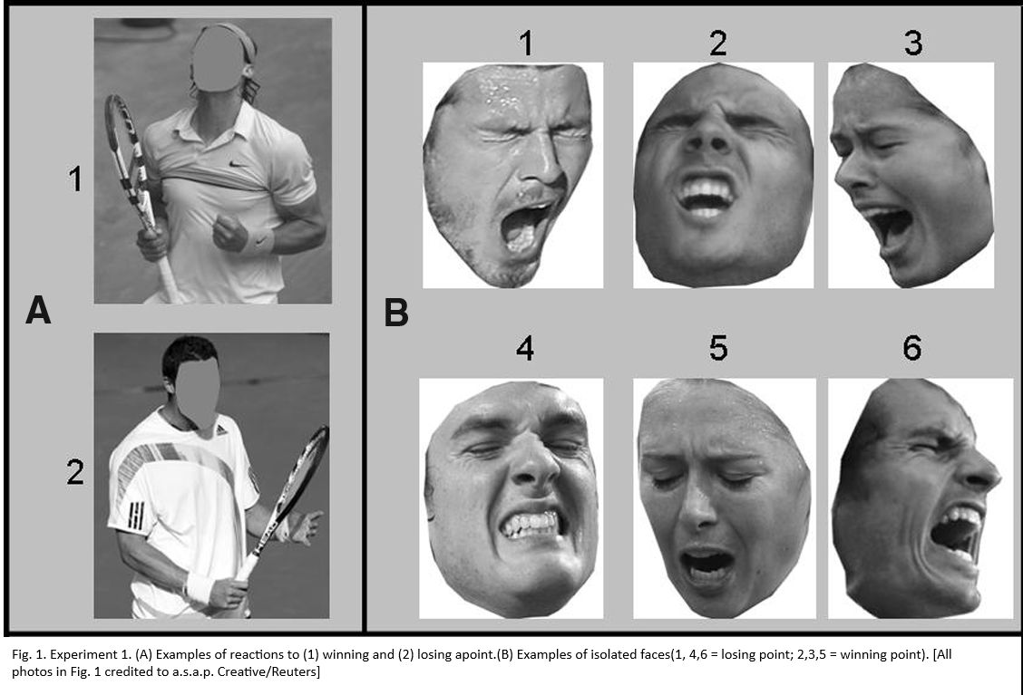
Etude d’Avezier et al. 2012 - 45 participants

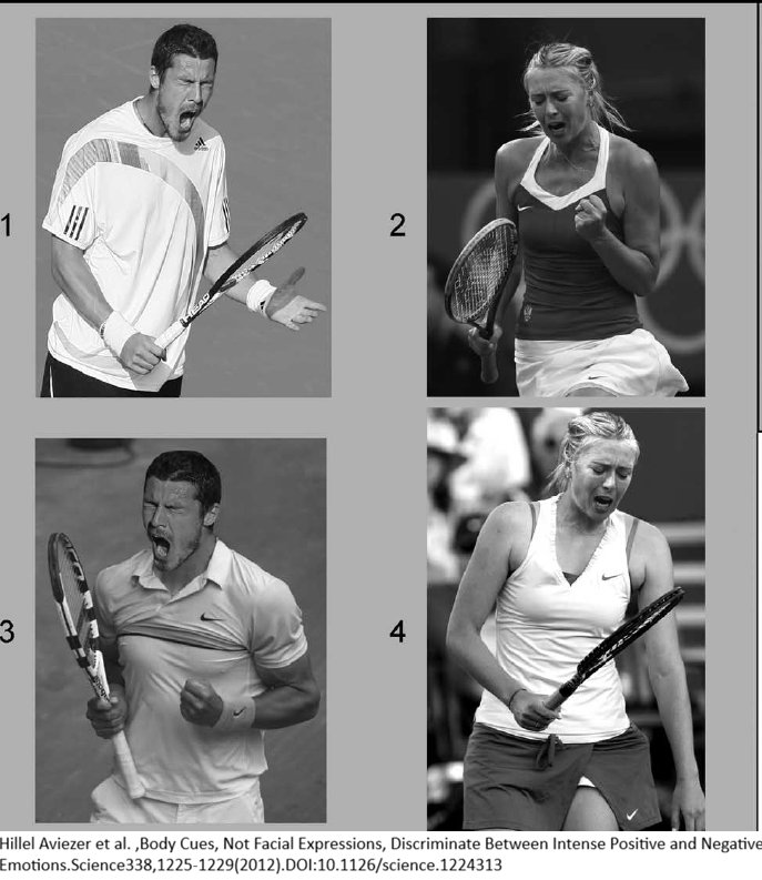
Exemple en Psychologie

- 45 participants - étude initiale - Avezier et al. en 2012 – Science ;

- 14 participants - réplication en 2018 - Camerer et al. – Nature ;

- 24 participants - réplication en 2023, Holzmeister et al. - Pre-data Collection Replication Report, OSF ;

- 194 participants - réplication de N. Pillaud en 2025 - Pillaud et al. 2025 – Emotion ;

- Réplication en live - une journée d’études - Université de Bordeaux : 62 membres de l’ESR;

-> Qu’est-ce qu’un petit nombre ? de 14 participants à 194 l’effet reste stable

Exemple en Psychologie

Implication de la taille d’effet

- la plus petite taille d’effet rapportée dans l’étude initiale est de :

- \(\eta^2_p\) = 0.74

- \(d\) = 3.37

Puissance statistique : éléments de définition

Probabilité de trouver un effet s’il existe

Puissance statistique : perspective historique

- J. Neyman & E. Pearson - 1933

- J. Cohen - 1962, 1988

- …

Puissance statistique : éléments de définition

	Rejet de \(H_0\)	Non-rejet de \(H_0\)
\(H_0\) correcte	Erreur de Type I (\(\alpha\))	Décision correcte (\(1 - \alpha\))
\(H_0\) incorrecte	Décision correcte (\(1 - \beta\))	Erreur de Type II (\(\beta\))

Tests d’hypothèse

On en utilise tout le temps en SHS :

khi2,
test-t,
corrélation,
régressions,
SEM,
etc.

Différentes tailles d’effet

\[ d = \frac{|mA - mB|}{SD_{pooled}}\]

- \(d\) de Cohen : indice de taille d’effet pour échantillons indépendants.

- \(mA\) & \(mB\) : sont les moyennes des groupes \(A\) et \(B\).

- \(SD_{pooled}\) : indice de dispersion (écart-type) commun des 2 groupes: \[SD_{pooled} = \sqrt {\frac {\sum{(x - mA)^2} + \sum{(x - mB)^2}}{nA + nB - 2}}\]

Avec \(mA\) & \(mB\), les moyennes des groupes \(A\) et \(B\) et \(nA\) & \(nB\) les effectifs des groupes A et B.

\[ \eta_p^2 = \frac {t^2}{t^2 + (nA + nB - 2)}\] - \(\eta_p^2\) : indice de taille d’effet pour échantillons indépendants.

- \(t\) : indice statistique du test \(t\) (aussi appelé \(t\) de Student).

- \(nA\) & \(nB\) : effectifs des groupes A et B.

\[ V = \sqrt {\frac{\chi^2}{n * k}} \]

- \(V\) : indice de taille d’effet pour 2 variables catégorielles à plusieurs modalités.

- \(\chi^2\) : indice statistique du test du \(\chi^2\).

- \(n\) : échantillon total.

- \(k\) : le plus petit nombre, soit de lignes, soit de colonnes, de la table de contingence.

Exemple 1 : un effet significatif, mais…

Test du \(khi²\) et taille d’effet (\(V\) de Cramer)

Fréquence de visite de sa mère biologique et le fait d’être au chômage


    Pearson's Chi-squared test

data:  chi2
X-squared = 34.423, df = 3, p-value = 1.613e-07

[1] 0.07695327

Puissance sur une petite taille d’effet

+--------------------------------------------------+
|                POWER CALCULATION                 |
+--------------------------------------------------+

Generic Chi-square Test

---------------------------------------------------
Hypotheses
---------------------------------------------------
  H0 (Null Claim)   : ncp = null.ncp 
  H1 (Alt. Claim)   : ncp > null.ncp 

---------------------------------------------------
Results
---------------------------------------------------
  Type 1 Error (alpha)   = 0.050
  Type 2 Error (beta)    = 0.000
  Statistical Power      = 1  <<

Exemple 2 : Un gros échantillon, mais…

L’exemple précédent portait sur 5813 observations.

Calcul de puissance a priori

+--------------------------------------------------+
|             SAMPLE SIZE CALCULATION              |
+--------------------------------------------------+

Chi-Square Test for Goodness-of-Fit or Independence

---------------------------------------------------
Hypotheses
---------------------------------------------------
  H0 (Null Claim)   : P[i,j] = P0[i,j] for all (i,j) 
  H1 (Alt. Claim)   : P[i,j] != P0[i,j] for some (i,j)

---------------------------------------------------
Results
---------------------------------------------------
  Total Sample Size      = 1844  << 
  Type 1 Error (alpha)   = 0.050
  Type 2 Error (beta)    = 0.200
  Statistical Power      = 0.8

Puissance statistique

Différents modèles, différents algorithmes

Exemple - t de Student

Test t et taille d’effet (\(d\) de Cohen) Satisfaction de la répartition des tâches ménagères comparaison hommes/femmes parmi les agriculteurs

t.test(DF_agri$OA_SATREP~DF_agri$MA_SEXE, var.equal=T)


    Two Sample t-test

data:  DF_agri$OA_SATREP by DF_agri$MA_SEXE
t = 2.3735, df = 92, p-value = 0.0197
alternative hypothesis: true difference in means between group 1 and group 2 is not equal to 0
95 percent confidence interval:
 0.1256708 1.4141843
sample estimates:
mean in group 1 mean in group 2 
       8.291667        7.521739

cohen.d(DF_agri$OA_SATREP, DF_agri$MA_SEXE)

Call: cohen.d(x = DF_agri$OA_SATREP, group = DF_agri$MA_SEXE)
Cohen d statistic of difference between two means
     lower effect upper
[1,]  -0.9   -0.5 -0.08

Multivariate (Mahalanobis) distance between groups
[1] 0.5
r equivalent of difference between two means
 data 
-0.24

Exemple - t de Student

Calcul de puissance a priori

power.t.student(d = -0.5,
                power = 0.80,
                alpha = 0.05,
                alternative = "two.sided",
                design = "independent")

+--------------------------------------------------+
|             SAMPLE SIZE CALCULATION              |
+--------------------------------------------------+

Student's T-Test (Independent Samples)

---------------------------------------------------
Hypotheses
---------------------------------------------------
  H0 (Null Claim) : d - null.d = 0 
  H1 (Alt. Claim) : d - null.d != 0 

---------------------------------------------------
Results
---------------------------------------------------
  Sample Size            = 64 and 64  <<
  Type 1 Error (alpha)   = 0.050
  Type 2 Error (beta)    = 0.199
  Statistical Power      = 0.801

Exemple - t de Student

Calcul de puissance a posteriori

power.t.test(ncp = 2.3735,
                df = 92,
                alpha = 0.05,
                alternative = "two.sided",
                plot = FALSE)

+--------------------------------------------------+
|                POWER CALCULATION                 |
+--------------------------------------------------+

Generic T-Test

---------------------------------------------------
Hypotheses
---------------------------------------------------
  H0 (Null Claim) : ncp = null.ncp 
  H1 (Alt. Claim) : ncp != null.ncp 

---------------------------------------------------
Results
---------------------------------------------------
  Type 1 Error (alpha)   = 0.050
  Type 2 Error (beta)    = 0.349
  Statistical Power      = 0.651  <<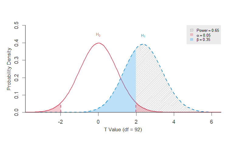

Exemple - t de Student

Test t et taille d’effet (\(d\) de Cohen) Satisfaction de la répartition des tâches ménagères selon la présence ou l’absence d’enfant de moins de 14ans dans le ménage, parmi les femmes

t.test(DF_500f$OA_SATREP~DF_500f$NBENF14_rec, var.equal=T)


    Two Sample t-test

data:  DF_500f$OA_SATREP by DF_500f$NBENF14_rec
t = -0.21736, df = 498, p-value = 0.828
alternative hypothesis: true difference in means between group 1 and group 2 is not equal to 0
95 percent confidence interval:
 -0.3816300  0.3056018
sample estimates:
mean in group 1 mean in group 2 
       7.864583        7.902597

cohen.d(DF_500f$OA_SATREP, DF_500f$NBENF14_rec)

Call: cohen.d(x = DF_500f$OA_SATREP, group = DF_500f$NBENF14_rec)
Cohen d statistic of difference between two means
     lower effect upper
[1,] -0.16   0.02   0.2

Multivariate (Mahalanobis) distance between groups
[1] 0.02
r equivalent of difference between two means
data 
0.01

Exemple - t de Student

Calcul de puissance a priori

power.t.student(d = 0.02,
                power = 0.80,
                alpha = 0.05,
                alternative = "two.sided",
                design = "independent")

+--------------------------------------------------+
|             SAMPLE SIZE CALCULATION              |
+--------------------------------------------------+

Student's T-Test (Independent Samples)

---------------------------------------------------
Hypotheses
---------------------------------------------------
  H0 (Null Claim) : d - null.d = 0 
  H1 (Alt. Claim) : d - null.d != 0 

---------------------------------------------------
Results
---------------------------------------------------
  Sample Size            = 39246 and 39246  <<
  Type 1 Error (alpha)   = 0.050
  Type 2 Error (beta)    = 0.200
  Statistical Power      = 0.8

Exemple - t de Student

Calcul de puissance a posteriori

power.t.test(ncp = -0.21736,
                df = 498,
                alpha = 0.05,
                alternative = "two.sided",
                plot = FALSE)

+--------------------------------------------------+
|                POWER CALCULATION                 |
+--------------------------------------------------+

Generic T-Test

---------------------------------------------------
Hypotheses
---------------------------------------------------
  H0 (Null Claim) : ncp = null.ncp 
  H1 (Alt. Claim) : ncp != null.ncp 

---------------------------------------------------
Results
---------------------------------------------------
  Type 1 Error (alpha)   = 0.050
  Type 2 Error (beta)    = 0.945
  Statistical Power      = 0.055  <<

Exemple - t de Student

Test t et taille d’effet (\(d\) de Cohen)

t.test(DF_f$OA_SATREP~DF_f$NBENF14_rec, var.equal=T)


    Two Sample t-test

data:  DF_f$OA_SATREP by DF_f$NBENF14_rec
t = -2.8853, df = 3263, p-value = 0.003937
alternative hypothesis: true difference in means between group 1 and group 2 is not equal to 0
95 percent confidence interval:
 -0.33378601 -0.06368395
sample estimates:
mean in group 1 mean in group 2 
       7.729233        7.927968

cohen.d(DF_f$OA_SATREP, DF_f$NBENF14_rec)

Call: cohen.d(x = DF_f$OA_SATREP, group = DF_f$NBENF14_rec)
Cohen d statistic of difference between two means
     lower effect upper
[1,]  0.03    0.1  0.17

Multivariate (Mahalanobis) distance between groups
[1] 0.1
r equivalent of difference between two means
data 
0.05

Exemple - t de Student

Calcul de puissance a priori

power.t.student(d = 0.1,
                power = 0.80,
                alpha = 0.05,
                alternative = "two.sided",
                design = "independent")

+--------------------------------------------------+
|             SAMPLE SIZE CALCULATION              |
+--------------------------------------------------+

Student's T-Test (Independent Samples)

---------------------------------------------------
Hypotheses
---------------------------------------------------
  H0 (Null Claim) : d - null.d = 0 
  H1 (Alt. Claim) : d - null.d != 0 

---------------------------------------------------
Results
---------------------------------------------------
  Sample Size            = 1571 and 1571  <<
  Type 1 Error (alpha)   = 0.050
  Type 2 Error (beta)    = 0.200
  Statistical Power      = 0.8

Exemple - t de Student

Calcul de puissance a posteriori

+--------------------------------------------------+
|                POWER CALCULATION                 |
+--------------------------------------------------+

Generic T-Test

---------------------------------------------------
Hypotheses
---------------------------------------------------
  H0 (Null Claim) : ncp = null.ncp 
  H1 (Alt. Claim) : ncp != null.ncp 

---------------------------------------------------
Results
---------------------------------------------------
  Type 1 Error (alpha)   = 0.050
  Type 2 Error (beta)    = 0.178
  Statistical Power      = 0.822  <<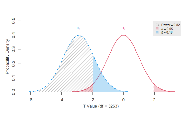

Pourquoi cette différence ?

500obs, effet non significatif (p>0.05), \(d\) = 0.02, \(Power\) = 0.06
3265obs, effet significatif (p<0.05), \(d\) = 0.1, \(Power\) = 0.82

Exemple - khi2

Test du \(khi²\) et taille d’effet (\(V\) de Cramer) Comparaison des réponses homme/femme sur l’aide aux devoirs

chi2<-table(DFp$EA_AID, DFp$MA_SEXE)
reschi<-chisq.test(chi2)
#reschi$expected

reschi


    Pearson's Chi-squared test

data:  chi2
X-squared = 510.29, df = 7, p-value < 2.2e-16

CramerV2<-cramer_v(DFp$EA_AID, DFp$MA_SEXE)
CramerV2

[1] 0.5392244

Exemple - khi2

Calcul de puissance a priori

+--------------------------------------------------+
|             SAMPLE SIZE CALCULATION              |
+--------------------------------------------------+

Chi-Square Test for Goodness-of-Fit or Independence

---------------------------------------------------
Hypotheses
---------------------------------------------------
  H0 (Null Claim)   : P[i,j] = P0[i,j] for all (i,j) 
  H1 (Alt. Claim)   : P[i,j] != P0[i,j] for some (i,j)

---------------------------------------------------
Results
---------------------------------------------------
  Total Sample Size      = 50  << 
  Type 1 Error (alpha)   = 0.050
  Type 2 Error (beta)    = 0.193
  Statistical Power      = 0.807

Exemple - khi2

Calcul de puissance a posteriori

+--------------------------------------------------+
|                POWER CALCULATION                 |
+--------------------------------------------------+

Generic Chi-square Test

---------------------------------------------------
Hypotheses
---------------------------------------------------
  H0 (Null Claim)   : ncp = null.ncp 
  H1 (Alt. Claim)   : ncp > null.ncp 

---------------------------------------------------
Results
---------------------------------------------------
  Type 1 Error (alpha)   = 0.050
  Type 2 Error (beta)    = 0.000
  Statistical Power      = 1  <<

Exemple - régressions linéaires

Modèle de régression linéaire


===============================================
                        Dependent variable:    
                    ---------------------------
                             OB_DEDUC          
-----------------------------------------------
MA_SEXE)2                    -0.338***         
                              (0.023)          
                                               
MA_AGEM_rec                   -0.001           
                              (0.001)          
                                               
AH_CS8)3                      -0.008           
                              (0.052)          
                                               
AH_CS8)4                      -0.004           
                              (0.048)          
                                               
AH_CS8)5                      -0.027           
                              (0.049)          
                                               
AH_CS8)6                       0.002           
                              (0.049)          
                                               
AH_CS8)7                      -0.040           
                              (0.071)          
                                               
AH_CS8)8                     -0.114**          
                              (0.056)          
                                               
Constant                     3.169***          
                              (0.069)          
                                               
-----------------------------------------------
Observations                   2,959           
R2                             0.104           
Adjusted R2                    0.102           
Residual Std. Error      0.533 (df = 2950)     
F Statistic          42.910*** (df = 8; 2950)  
===============================================
Note:               *p<0.1; **p<0.05; ***p<0.01


Call:
lm(formula = DFp$OB_DEDUC ~ factor(DFp$MA_SEXE) + DFp$MA_AGEM_rec + 
    factor(DFp$AH_CS8))

Standardized Coefficients::
         (Intercept) factor(DFp$MA_SEXE)2      DFp$MA_AGEM_rec 
                  NA         -0.299676843         -0.008885231 
 factor(DFp$AH_CS8)3  factor(DFp$AH_CS8)4  factor(DFp$AH_CS8)5 
        -0.004340916         -0.003093925         -0.020698836 
 factor(DFp$AH_CS8)6  factor(DFp$AH_CS8)7  factor(DFp$AH_CS8)8 
         0.001123818         -0.013410187         -0.058553337

Exemple - régressions linéaires

Puissance a priori sur l’ensemble du modèle

power.f.regression(r.squared = 0.102,
                   k.total = 8,
                   power = 0.80,
                   alpha = 0.05)

+--------------------------------------------------+
|             SAMPLE SIZE CALCULATION              |
+--------------------------------------------------+

Linear Regression (F-Test)

---------------------------------------------------
Hypotheses
---------------------------------------------------
  H0 (Null Claim) : R-squared = 0 
  H1 (Alt. Claim) : R-squared > 0 

---------------------------------------------------
Results
---------------------------------------------------
  Sample Size          = 141  <<
  Type 1 Error (alpha) = 0.050
  Type 2 Error (beta)  = 0.197
  Statistical Power    = 0.803

Exemple - régressions linéaires

Puissance a posteriori

power.f.regression(r.squared = 0.102,
                   k.total = 8,
                   n = 2959,
                   alpha = 0.05)

+--------------------------------------------------+
|                POWER CALCULATION                 |
+--------------------------------------------------+

Linear Regression (F-Test)

---------------------------------------------------
Hypotheses
---------------------------------------------------
  H0 (Null Claim) : R-squared = 0 
  H1 (Alt. Claim) : R-squared > 0 

---------------------------------------------------
Results
---------------------------------------------------
  Sample Size          = 2959
  Type 1 Error (alpha) = 0.050
  Type 2 Error (beta)  = 0.000
  Statistical Power    = 1  <<

Exemple - régressions linéaires

Puissance a priori pour une variable

+--------------------------------------------------+
|             SAMPLE SIZE CALCULATION              |
+--------------------------------------------------+

Linear Regression Coefficient (T-Test)

---------------------------------------------------
Hypotheses
---------------------------------------------------
  H0 (Null Claim) : beta - null.beta = 0 
  H1 (Alt. Claim) : beta - null.beta != 0 

---------------------------------------------------
Results
---------------------------------------------------
  Sample Size            = 81  <<
  Type 1 Error (alpha)   = 0.050
  Type 2 Error           = 0.198
  Statistical Power      = 0.802

Exemple - régressions linéaires

Puissance a posteriori pour une variable

+--------------------------------------------------+
|                POWER CALCULATION                 |
+--------------------------------------------------+

Linear Regression Coefficient (T-Test)

---------------------------------------------------
Hypotheses
---------------------------------------------------
  H0 (Null Claim) : beta - null.beta = 0 
  H1 (Alt. Claim) : beta - null.beta != 0 

---------------------------------------------------
Results
---------------------------------------------------
  Sample Size            = 2959
  Type 1 Error (alpha)   = 0.050
  Type 2 Error           = 0.000
  Statistical Power      = 1  <<

Exemple - régressions logistiques

Coefficients pour niveau diplôme >BAC+2

Coefficients standardisés & Odds Ratios
Parameter	Std_Odds_Ratio	CI	CI_low	CI_high
(Intercept)	12.353	0.950	5.137	32.531
MA_AGEM_rec	0.656	0.950	0.467	0.914
MA_SEXE2	0.006	0.950	0.003	0.014
MC_DIPLOME2	0.898	0.950	0.172	4.997
MC_DIPLOME3	0.078	0.950	0.012	0.438
MC_DIPLOME4	0.490	0.950	0.180	1.274
MC_DIPLOME5	0.285	0.950	0.058	1.331
MC_DIPLOME6	0.221	0.950	0.019	1.634
MC_DIPLOME7	0.478	0.950	0.092	2.225
MC_DIPLOME8	0.293	0.950	0.085	0.973

Exemple - régressions logistiques

Taille d’effet pour niveau diplôme >BAC+2

# Calcul de "base.prob" :
base.prob = 12.35/(1+12.35)
base.prob

[1] 0.9250936

# taille d'effet du prédicteur niveau de diplome = 8 (pseudo-R2)
pseudo_r2_dip8

'log Lik.' 0.58883 (df=9)

Exemple - régressions logistiques

Puissance a priori pour niveau diplôme >BAC+2

power.z.logistic(odds.ratio = 0.29,
                 base.prob = 0.925,
                 r.squared.predictor = 0.589,
                 power = 0.80,
                 alpha = 0.05,
                 alternative = "two.sided",
                 distribution = "normal")

+--------------------------------------------------+
|             SAMPLE SIZE CALCULATION              |
+--------------------------------------------------+

Logistic Regression Coefficient (Wald's Z-Test)

  Method          : Demidenko (Variance Corrected)
  Predictor Dist. : Normal

---------------------------------------------------
Hypotheses
---------------------------------------------------
  H0 (Null Claim) : Odds Ratio = 1
  H1 (Alt. Claim) : Odds Ratio != 1

---------------------------------------------------
Results
---------------------------------------------------
  Sample Size          = 173  <<
  Type 1 Error (alpha) = 0.050
  Type 2 Error (beta)  = 0.199
  Statistical Power    = 0.801

Exemple - régressions logistiques

Puissance a posteriori pour niveau diplôme >BAC+2

power.z.logistic(odds.ratio = 0.29,
                 base.prob = 0.925,
                 r.squared.predictor = 0.589,
                 n = 471,
                 alpha = 0.05,
                 alternative = "two.sided",
                 distribution = "normal")

+--------------------------------------------------+
|                POWER CALCULATION                 |
+--------------------------------------------------+

Logistic Regression Coefficient (Wald's Z-Test)

  Method          : Demidenko (Variance Corrected)
  Predictor Dist. : Normal

---------------------------------------------------
Hypotheses
---------------------------------------------------
  H0 (Null Claim) : Odds Ratio = 1
  H1 (Alt. Claim) : Odds Ratio != 1

---------------------------------------------------
Results
---------------------------------------------------
  Sample Size          = 471
  Type 1 Error (alpha) = 0.050
  Type 2 Error (beta)  = 0.001
  Statistical Power    = 0.999  <<

Quelques remarques

- Les variables de pondération peuvent être intégrées aux modèles

- Le calcul de puissance implique de bien connaître son sujet (et notamment la taille d’effet envisagée)

- Surestimation de la taille d’effet dans la littérature

Conclusion

Les petits nombres, c’est relatif
Des trop gros nombres ne sont pas toujours avantageux

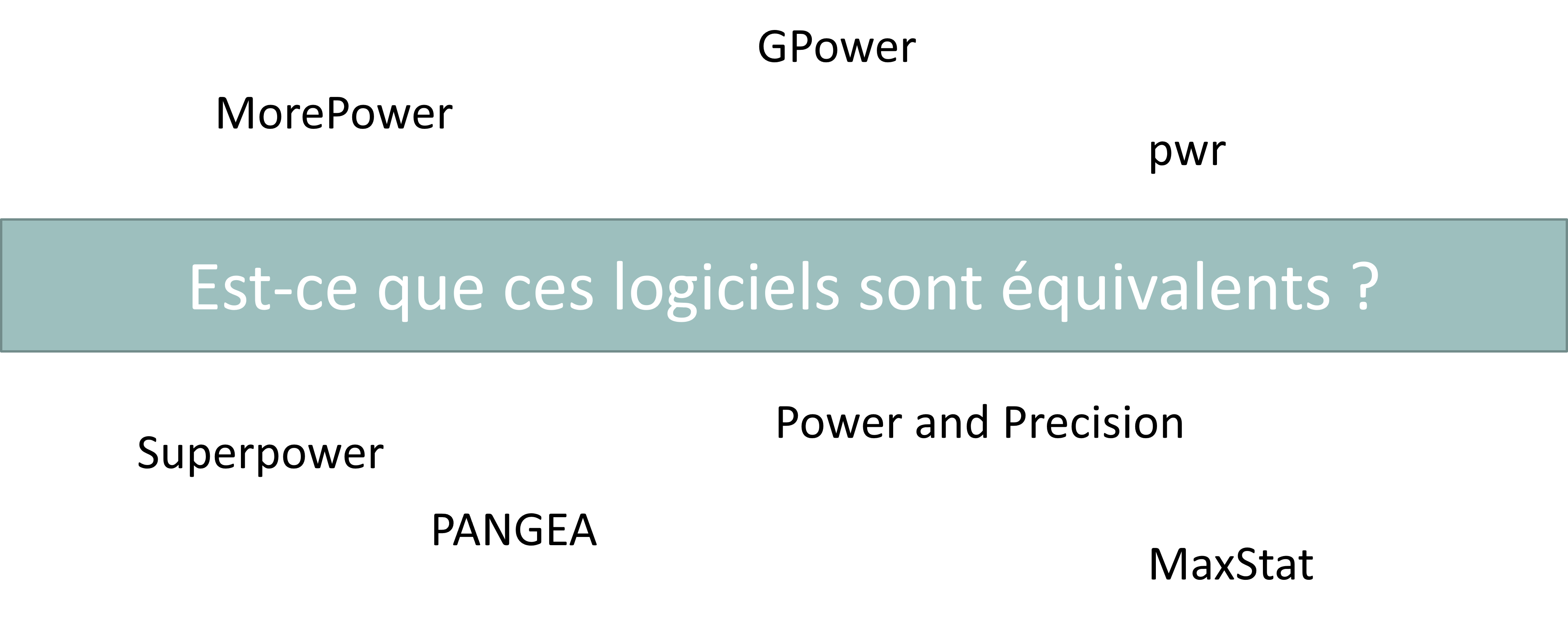
Ressources en ligne - designs simples

Pour des designs simples (ANOVA, régressions, etc.) :

**G*Power** - le logiciel : https://www.psychologie.hhu.de/arbeitsgruppen/allgemeine-psychologie-und-arbeitspsychologie/gpower
MorePower - le dépôt github : https://github.com/LewisPeacockLab/MorePower/blob/main/README.md
PANGEA - le dépôt github : https://github.com/jake-westfall/pangea
powerMediation - le package R : https://weiliang.r-universe.dev/powerMediation/doc/manual.html
Power and Precision - le logiciel : https://power-analysis.com/?utm_source=softwareworld.co&utm_medium=referral
pwr - le package R : https://github.com/heliosdrm/pwr & le lien CRAN : https://cran.r-project.org/web/packages/pwr/index.html
pwrss - le package R : https://cran.r-project.org/web/packages/pwrss/vignettes/examples.html#1_Generic
Superpower - le package R : https://cran.r-project.org/web/packages/Superpower/vignettes/intro_to_superpower.html

Ressources en ligne - SEM & modèles longitudinaux

Pour des SEM (Structural Equation Models) :

semPower - dépôt github : https://github.com/moshagen/semPower & le lien CRAN : https://cran.r-project.org/web/packages/semPower/index.html
simsem - le package R : https://simsem.org/

Pour des modèles mixtes / longitudinaux :

longpower - le package R : https://cran.r-universe.dev/longpower/doc/manual.html
powerlmm - le package R : https://rpsychologist.com/introducing-powerlmm
simr - le package R : https://cran.r-universe.dev/simr/doc/manual.html
webpower - le logiciel en ligne : https://webpower.psychstat.org/wiki/ & le package R : https://cran.r-project.org/web//packages//WebPower/index.html

Pour des analyses de survie :

powerSurvEpi - le package R : https://weiliang.r-universe.dev/powerSurvEpi

Bibliographie

Aviezer, Hillel, Yaacov Trope, and Alexander Todorov. 2012. “Body Cues, Not Facial Expressions, Discriminate Between Intense Positive and Negative Emotions.” Science 338 (6111): 1225–29. https://doi.org/10.1126/science.1224313.

Biau, David Jean, Brigitte M. Jolles, and Raphaël Porcher. 2010. “P Value and the Theory of Hypothesis Testing: An Explanation for New Researchers.” Clinical Orthopaedics & Related Research 468 (3): 885–92. https://doi.org/10.1007/s11999-009-1164-4.

Caldwell, Aaron R., Daniël Lakens, Chelsea M. Parlett-Pelleriti, Guy Prochilo, and Frederik Aust. n.d. Power Analysis with Superpower. Accessed January 21, 2026. https://aaroncaldwell.us/SuperpowerBook/.

Camerer, Colin F., Anna Dreber, Felix Holzmeister, Teck-Hua Ho, Jürgen Huber, Magnus Johannesson, Michael Kirchler, et al. 2018. “Evaluating the Replicability of Social Science Experiments in Nature and Science Between 2010 and 2015.” Nature Human Behaviour 2 (9): 637–44. https://doi.org/10.1038/s41562-018-0399-z.

Campbell, Jamie I. D., and Valerie A. Thompson. 2012. “MorePower 6.0 for ANOVA with Relational Confidence Intervals and Bayesian Analysis.” Behavior Research Methods 44 (4): 1255–65. https://doi.org/10.3758/s13428-012-0186-0.

Cohen, Jacob. 1962. “The Statistical Power of Abnormal-Social Psychological Research: A Review.” The Journal of Abnormal and Social Psychology 65 (3): 145–53. https://doi.org/10.1037/h0045186.

———. 2013. Statistical Power Analysis for the Behavioral Sciences. 0th ed. Routledge. https://doi.org/10.4324/9780203771587.

Faul, Franz, Edgar Erdfelder, Axel Buchner, and Albert-Georg Lang. 2009. “Statistical Power Analyses Using G*Power 3.1: Tests for Correlation and Regression Analyses.” Behavior Research Methods 41 (4): 1149–60. https://doi.org/10.3758/BRM.41.4.1149.

Faul, Franz, Edgar Erdfelder, Albert-Georg Lang, and Axel Buchner. 2007. “G*Power 3: A Flexible Statistical Power Analysis Program for the Social, Behavioral, and Biomedical Sciences.” Behavior Research Methods 39 (2): 175–91. https://doi.org/10.3758/BF03193146.

Iddi, Samuel, and Michael C. Donohue. 2022. “Power and Sample Size for Longitudinal Models in R – The Longpower Package and Shiny App.” The R Journal 14 (1): 264–82. https://doi.org/10.32614/RJ-2022-022.

Ioannidis, John P. A. 2005. “Why Most Published Research Findings Are False.” PLoS Medicine 2 (8): e124. https://doi.org/10.1371/journal.pmed.0020124.

Jak, Suzanne, Terrence D. Jorgensen, Mathilde G. E. Verdam, Frans J. Oort, and Louise Elffers. 2020. “Analytical Power Calculations for Structural Equation Modeling: A Tutorial and Shiny App.” Behavior Research Methods 53 (4): 1385–1406. https://doi.org/10.3758/s13428-020-01479-0.

Krivitsky, Pavel N., and Mark S. Handcock. 2014. “A Separable Model for Dynamic Networks.” Journal of the Royal Statistical Society Series B: Statistical Methodology 76 (1): 29–46. https://doi.org/10.1111/rssb.12014.

Lakens, Daniël, and Aaron R. Caldwell. 2021. “Simulation-Based Power Analysis for Factorial Analysis of Variance Designs.” Advances in Methods and Practices in Psychological Science 4 (1): 2515245920951503. https://doi.org/10.1177/2515245920951503.

Lakens, Daniël, and Ellen R. K. Evers. 2014. “Sailing From the Seas of Chaos Into the Corridor of Stability: Practical Recommendations to Increase the Informational Value of Studies.” Perspectives on Psychological Science 9 (3): 278–92. https://doi.org/10.1177/1745691614528520.

Lenhard, Wolfgang, and Alexandra Lenhard. 2017. “Computation of Effect Sizes.” Unpublished. https://doi.org/10.13140/RG.2.2.17823.92329.

Moshagen, Morten, and Martina Bader. 2023. “semPower: General Power Analysis for Structural Equation Models.” Behavior Research Methods 56 (4): 2901–22. https://doi.org/10.3758/s13428-023-02254-7.

———. 2025. Power Analysis for Structural Equation Models: semPower 2 Manual. https://moshagen.github.io/semPower/.

Neyman, Jerzy, and Egon Sharpe Pearson. 1933. “IX. On the Problem of the Most Efficient Tests of Statistical Hypotheses.” Philosophical Transactions of the Royal Society of London. Series A, Containing Papers of a Mathematical or Physical Character 231 (694-706): 289–337. https://doi.org/10.1098/rsta.1933.0009.

Nuzzo, Regina. 2014. “Scientific Method: Statistical Errors.” Nature 506 (7487): 150–52. https://doi.org/10.1038/506150a.

Zhang, Zhiyong, and Ke-Hai Yuan. 2018. Practical Statistical Power Analysis Using Webpower and R. ISDSA Press. https://doi.org/10.35566/power.